ERP Tutorial 13 — Demand Forecast: Backtest Before You Trust

Twelve tutorials in, this series has treated demand as a given — sales orders arrive, MRP explodes them, capacity absorbs them. This tutorial introduces the tool that looks the other way in time: Demand Forecast, new under ERP → Planning, sitting right beside the MRP Workbench it feeds.

The Idea: Backtest Before You Trust

The page's method is honest by construction. It takes an item's monthly demand history, then runs four classic forecasting methods — Naive (next month = last month), 3-Month Moving Average, Weighted MA (3-2-1), and Exponential Smoothing (α=0.3) — through a one-step-ahead backtest: each method predicts months that already happened, using only the data that existed at the time, and gets scored by MAPE (mean absolute percentage error). The method that would have missed least wins the 🥇 and gets to make the real forecast: three months ahead, with an error band derived from its own backtest misses.

What Honest Looks Like on Thin Data

First, the anti-demo. Pick ITM-001, the SmartBar Pro 500:

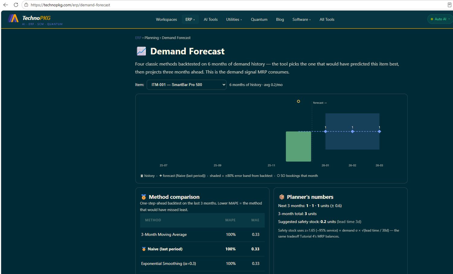
Average demand 0.2 units a month, a single bar on the chart. All four methods tie at 100% MAPE, and the projection is a flat line of ones. That's not a failure — it's the correct answer. A forecasting tool that produced a confident curve from one data point would be lying, and this one doesn't.

What It Does With Real History

Now switch to ITM-005, the Speaker Cabinet:

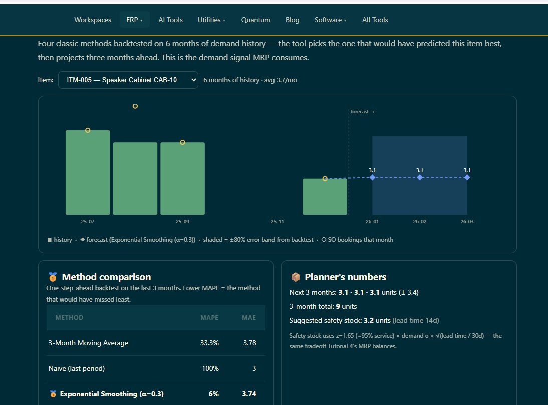
The cabinet's demand is lumpy — strong months, then a collapse. The backtest exposes each method's character: Naive chases the last observation and gets whipsawed (100% MAPE); the Moving Average smooths but drags old highs along (33%); Exponential Smoothing wins at 6%, because its slowly-decaying level absorbs the collapse without either chasing it or ignoring it. So the forecast uses SES: 3.1 units a month, ±3.4. Yes, the band is wider than the forecast — that's the tool being frank about a volatile item rather than faking precision.

The Planner's Numbers

The right-hand panel converts the statistics into decisions: a 3-month total (9 units) to size the plan, and a suggested safety stock of 3.2 units computed as z=1.65 (~95% service) × demand σ × √(lead time ÷ 30 days) — using the cabinet's real 14-day PrecisionParts lead time from the Item Master (Tutorial 10). Longer lead time, more variability, more buffer: the exact tradeoff Tutorial 4's MRP balances, now with the arithmetic visible.

One more detail worth noticing on the chart: the small orange rings mark actual sales-order bookings per month, drawn against the recorded demand bars. When rings and bars diverge, that's a data-quality conversation waiting to happen — the forecast is only as good as the history feeding it.

Where It Fits in the Series

Follow the flow end to end now: Forecast → S&OP → MRP → Work Orders → Shipments. This page produces the demand signal; Tutorial 5's S&OP consensus commits to it; Tutorial 4's MRP explodes it through the BOMs of Tutorial 7; Tutorial 6's work orders build it within Tutorial 9's capacity; Tutorial 11 ships it. The MRP Workbench even lists "Moving Average Forecast" and "Exponential Smoothing" among its planning algorithms — this page is where you can watch those same methods compete on evidence before trusting one in a planning run.

Try It Yourself

1. Open ERP → Demand Forecast and flip through the items — watch the 🥇 change hands depending on whether an item's demand trends, wobbles, or barely exists.
2. On ITM-005, check the arithmetic: does the 3-month total equal 3 × the monthly forecast?
3. Compare the suggested safety stock across two items with different lead times — same formula, different buffers.
4. Find a month where the orange ring sits far from its bar, and ask why bookings and recorded demand disagree.

Next up: Tutorial 14 — the BOM Builder, where the structures every plan explodes through stop being read-only.

Comments (0)